
We use cookies to help us deliver and improve this site. By clicking Confirm or by continuing to use the site, you agree to our use of cookies. For more information see our Cookie Policy.
Centrifugal Pump Selection
In choosing a pump, you firstly need to select a pump appropriate for your application. Centrifugal or positive displacement? Is the fluid corrosive? Does it have entrained solids? Does it need to be contained? However, having made those decisions, and if you have identified centrifugal pump technology as being the most suitable, how do you select a model to give the required performance?
How to read a centrifugal pump curve
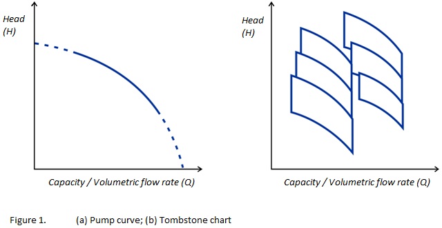
Historically, pumps were used to raise water for irrigation or drainage purposes. It was important that the pump was capable of lifting the water from the lower to the higher level. The delivery height became known as the differential head (or simply head) and, despite the vastly extended range of modern-day pumping applications, this term is still used to characterise pump performance. Nowadays, it relates more to the difference in pressure between the pump’s inlet and outlet and this can be affected by pipeline design and valve configurations. As the pressure a centrifugal pump has to overcome increases, the discharge flow decreases until, at a certain head, the output drops to zero. Conversely, with no head to work against, a pump can achieve the maximum possible output allowed by its design, impeller selection and rotational speed. The range of performance between these two points is specified in a pump curve (Figure 1a).
For a particular pump design, the performance can be modified by fitting a different impeller and/or by operating it at a different rotational speed. Manufacturers often show the range of possible performances in a ‘Tombstone’ chart (Figure 1b). This illustrates the head pressure and capacities covered by a pump design at a number of set rotational speeds, with a range of impeller sizes and different pump casing designs. The upper line of each segment or tombstone is the actual pump curve at the specified speed, impeller size and casing design.
What is the system curve?
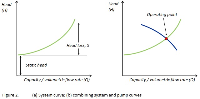
The pump curve describes how a centrifugal pump performs in isolation from plant equipment. How it operates in practice is determined by the resistance of the system it is installed in: restrictions in the pipework and downstream frictional losses as well as static inlet or outlet pressures. A graphical representation of these factors is called the system curve (Figure 2a). This shows how the head pressure (at the location to be occupied by the pump) increases with increasing throughput.
What varies the system curve?
A key component of the system curve is the head loss resulting from frictional effects as fluid is forced through downstream pipework. This arises from valves, junctions, elbows, changes in pipeline diameter, and friction between the fluid and the pipe walls. It is usually calculated using the Darcy-Weisbach equation:
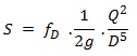
Where the head loss increases to the square of the volumetric flow rate (hence system curves are parabolic); is the Darcy-Weissbach frictional factor, is the pipe diameter and is the local acceleration due to gravity.
There can also be a fixed component to the system curve, introduced by any inherent differences in pressure between the fluid’s source and its discharge. This is called the static head and, in the conventional sense, is comparable to pumping the fluid to a higher (or lower) reservoir.
What is the operating point?
By plotting the pump and system curves on the same graph (Figure 2b), the intersection of the lines identifies the flow rate you can expect from the pump in this configuration. This intersection is called the operating point. If the lines do not intersect the pump is not suitable for your application.
Where is the most stable operating section of the pump’s curve?
A centrifugal pump has a best efficiency point (BEP) somewhere on its pump curve. These are the precise conditions, determined by the manufacturer, where the pump operates with greatest efficiency and at which it can be expected to have maximum working life and experience lower maintenance. Ideally, when choosing a pump, you should attempt to match the operating point and best efficiency points. Over the lifetime of the pump this can have considerable cost benefits. In practice, it is acceptable to match the operating point to within ±10% of the best efficiency point.
A pump operating at a lower capacity is often said to be “operating to the left of the curve” and at a higher capacity is termed “operating to the right of the curve”. These correspond to the relative positions on the pump curve on either side of the BEP.
What happens if you run too far left of curve
To the left of the BEP, a pump’s throughput is lower than its design specification and the fluid may not flow correctly through the system. There is a danger of recirculation in both the pump’s inlet and outlet. This can lead to vibration and seal wear.
Also, with a low flow, there can be problems with heat build-up. Heat is produced by the driving motor and by friction in the pump itself. This heat normally dissipates through the pumped fluid but under low flow conditions this may not occur efficiently enough to prevent overheating. The impeller, pump casing and bearings of a centrifugal pump are precisely engineered with minimum clearances to reduce losses and maximise efficiency. At higher temperatures, the gaps between these rapidly moving components is reduced still further and any contact will result in wear and potential damage.
What happens if you run too far right of curve
At the right-hand side of the BEP, a pump’s throughput is higher than its design specification and there is a danger of cavitation in the impeller.
Cavitation is a process whereby bubbles of vapour, formed when a fluid is under low pressure, spontaneously collapse as they are transported back into a region of higher pressure. In a centrifugal pump the fluid’s pressure is at a minimum at the eye of the impeller. If the pressure here is below the saturated vapour pressure of the fluid, bubbles are formed which pass on into and through the impeller vanes. The fluid pressure increases as the fluid is discharged and the bubbles implode. The repeated shock waves can be a significant cause of wear and metal fatigue on impellers and pump cases.
The higher discharge may also result in vibration and noise in the pump, placing greater strain on its drive shaft and other components, and also in downstream pipework. This can lead to greater maintenance costs and a higher incidence of pump failures.
What are the Affinity Laws?
The Affinity Laws are a set of relationships that show how a pump’s capacity, head and power are determined by the rotational speed or diameter of its impeller. They allow you to extrapolate from the specified pump curve and predict how the pump will perform at a different shaft speed or with a smaller (or larger) impeller installed.
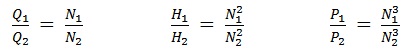
Fluid enters the rapidly rotating impeller along its axis and is cast out by centrifugal force along its circumference through the impeller’s vane tips. The output or volumetric flow of the pump (Q) is linearly related to the rotational speed of the impeller (N). In addition, the head (H) is proportional to the square of the impeller’s rotational speed, and the power requirements (P) to its cube:
![]()
These three relationships lead to the first set of Affinity Laws. Knowing the volumetric flow (Q1), head (H1) and power (P1) of a pump at one rotational speed (N1), you can use these relationships to estimate how it will perform (Q2 , H2 , P2) at a different speed (N2).
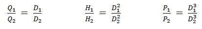
In the same way, the volumetric flow of the pump (Q) is linearly related to impeller diameter (D), the head (H) is proportional to its square, and the power requirements (P) to its cube:
![]()
So, if you know the capacity (Q1), head (H1) and power (P1) with one size of impeller (D1) installed in the pump, you can use a second set of Affinity Laws to estimate how it will perform (Q2 , H2 , P2) with a differently sized impeller (D2).
It is important to note that different sizes of impellers may not have the same efficiencies. Predictions using this set of Affinity Laws may not be as accurate as those derived from changes in rotational speed using the first set of laws.
Summary
To select the right pump for an application, it is important to understand both system and pump curves. The system curve describes the increase in head resulting from increasing fluid flow through the pipework and other equipment in your plant. The pump curve describes the relationship between the rate of fluid flow and head for the pump itself. When plotted on the same graph, the point at which the system curve and pump curves intersect is called the operating point – it identifies the capacity you can expect from the pump in this particular configuration. Ideally, you should choose a pump where the operating point matches the point of maximum efficiency on the pump curve (BEP). The Affinity Laws allow you to predict how a pump will perform at different rotational speeds or with an alternative impeller installed.